Tatsuki Ogino
1. Introduction
We have been able to execute a 3-dimensional global magnetohydrodynamic
(MHD) simulation of the interaction between the solar wind and earth's
magnetosphere in order to study the structure and dynamics of the
magnetosphere on a variety of computers using a fully vectorized MHD code.
Among the computers we have used are: CRAY Y-MP, Fujitsu VP-2600, Hitachi S820,
and NEC SX-3. This flexibility of using many different computers allowed us
to work together with many scientists executing our computer simulations.
However, as vector parallel and massively parallel supercomputers have come
into the simulation community, a number of different approaches are now being
used. Many simulation scientists have lost their common language and are being
forced to speak new dialects.
We began to use the vector parallel supercomputer, Fujitsu VPP500, in the
Computer Center of Nagoya University in 1995 and have succeeded in
rewriting our 3-dimensional global MHD simulation code in VPP Fortran to
achieve a high performance of over 17 Gflops. Moreover, we have used a new
supercomputer, the Fujitsu VPP5000/56 since last December to achieve a higher
performance of over 400 Gflops in VPP Fortran. However, the MHD code in VPP
Fortran cannot achieve such a high performance using other
supercomputers such as Hitachi SR8000 and NEC SX-5. Thus we face a difficult
problem in collaborating in computer simulations with other scientists even
in our domestic universities. We very much hope to recover the ability to
have a common language in the supercomputer world. Recent candidates for this
common language appear to be High Performance Fortran (HPF) and Message Passing
Interface (MPI). We look forward to the time when we can use these compilers
in supercomputers.
Last year I heard from some engineers in Japanese supercomputer companies that
they had tried to develop an extended version of HPF created by the Japanese
HPF Association (JAHPF) to supply the new HPF compiler in the near future.
I was very interested in this information because the performance of the
original HPF was questionable and we want to test this performance by ourselves.
Since last June, we have had the opportunity to use HPF/JA (an extended version
of HPF) with a supercomputer of the vector-parallel type, Fujitsu VPP5000/56.
We immediately began to translate our 3-dimensional MHD simulation code for
the Earth's magnetosphere from VPP Fortran to HPF/JA. The MHD code was fully
vectorized and fully parallelized in VPP Fortran. We successfully rewrote
the code from VPP Fortran to HPF/JA in three weeks,
and needed an additional two weeks to perform a final verification of the
calculation results. The entire performance and capability of the HPF MHD code
are shown to be almost comparable to those of the VPP Fortran in a typical
simulation by Fujitsu VPP5000/56.
2. From VPP Fortran to HPF/JA
We asked the Computer Center of Nagoya University to begin to use HPF in
their supercomputer as soon as possible. Last June, we had an
opportunity to hear a lecture on HPF by a Fujitsu engineer and we began
to use HPF/JA on the Fujitsu VPP5000. We heard that the use of HPF was
not very successful in the USA and Europe, and that users would rather
abandon the usage of HPF due to its difficulty to achieving a high
performance. However, we have high expectations of HPF/JA because
supercomputer companies in Japan have had good experiences with compilers in
operating vector-parallel machines. I will decide to translate our MHD code
from VPP Fortran to HPF if half the performance of VPP Fortran can be obtained
using HPF. We have experience in fully vectorizing and parallelizing several
test programs and 3-dimensional global MHD codes for the earth's magnetosphere
using VPP Fortran. Thus I had the impression that we could obtain good
performance by translating the MHD codes from VPP Fortran to HPF/JA after
hearing the HPF lecture. The main points are summarized as follows,
Fortran programs using VPP Fortran can be be directly rewritten using
HPF/JA owing to (1)-(3) keeping their original styles. If unnecessary
communication could be completely stopped by (5), the efficiency of
parallelization could be greatly improved. We can use the instructions
to stop unnecessary communication if the calculation results don't
change with insertion of the instructions. Generally it is very difficult
for the parallel compiler to know whether the communication is needed or not
in advance because variables might be rewritten at anytime. Therefore
unnecessary communication that users cannot be aware of frequently happens
and the efficiency of parallelization cannot increase. That is, the compiler
just compiles programs considering all cases; it cannot provide a good solution
if there exists any uncertain portion, and therefore unexpected and unnecessary
communication very often occurs in the execution of a program.
We can succeed in parallelization of the MHD program even in the
worst case because the high speed alternation in the division directions
by (4) can solve almost all the difficulties of parallelization in the MHD
program, e.g. in the treatment of boundary conditions. We could fully
parallelize our MHD code by using the function of division alternation when
we used the ADETRAN compiler of Matsusita Electric Co. We obtained an efficiency
of parallelization over 85% using the ADETRAN massively parallel computer with
256 processors. Moreover, we can execute parallel computation in maximum,
minimum and summation by using a "reduction" sentence in HPF/JA. Because we
had high expectations for translating programs from VPP Fortran to HPF/JA,
we soon began to rewrite several test programs and the 3-dimensional MHD code.
3. Comparison of Processing Capability by VPP Fortran and HPF/JA
Our aim is to translate the 3-dimensional global MHD simulation code for
interaction between the solar wind and the earth's magnetosphere from
VPP Fortran to HPF/JA and to achieve an efficiency more than 50% over VPP Fortran.
In the global MHD simulation, the MHD and Maxwell's equations are solved by
the modified leap-frog method as an initial value and boundary value problem to
study the response of the magnetosphere to variations of the solar wind and the
interplanetary magnetic field (IMF). Because the external boundary is put in
a distant region to avoid its influence on the boundary condition and the tail
boundary is extended to look at structure of the distant tail, then higher
spatial resolution is required to obtain numerically accurate results.
Therefore, the number of 3-dimensional grid points increases up to the limit
of computers.
Examples of MHD simulations of the solar wind-magnetosphere interaction
are shown in Figures 1 and 2. Figure 1 shows the 3-dimensional structure
of magnetic field lines under steady state conditions for the earth's
magnetosphere when the IMF is northward and duskward . A dawn-dusk
asymmetry appears in the structure of magnetic field lines because
magnetic reconnection at the magnetopause occurs in the high latitude
tail on the dusk side in the northern hemisphere and on the dawn side
in the southern hemisphere. Figure 2 shows a snapshot of the earth's
magnetosphere obtained by 3-dimensional global MHD simulation when
the ACE satellite is monitoring the upstream solar wind and IMF every
1 minute. These data were used as input to the simulation. This simulation
is one of the fundamental studies in the international space weather program
designed to develop numerical models and to understand the variations in the
solar-terrestrial environment from moment to moment. It requires 50-300 hours
of computation time to execute these 3-dimensional global MHD simulations of
the earth's magnetosphere even by VPP5000/56.
Table 1 shows the comparison of computer processing capabilities of
VPP Fortran and HPF/JA by using a 3-dimensional global MHD code for
the solar wind-magnetosphere interaction run on the Fujitsu
VPP5000/56. Both the Fortran codes are fully vectorized and fully
parallelized, and are adjusted to reach the maximum performance
using the results of several test runs applying practical simulations.
The table includes the number of PEs (Processing Elements), 3-dimensional grid
points except for the boundary, cpu time (sec) to execute and advance of one
time step, computation speed (Gflops) and computation speed per PE (Gflops/PE)
for both VPP Fortran and HPF/JA.
The characteristics of the Fujitsu VPP5000/56 in the Computer Center of
Nagoya University are as follows,
As is known from Amdahl's law, it is quite important to fully vectorize
in all inner do loops and to fully parallelize in all outer do loops
in order to increase the efficiency of vectorization and parallelization
performance. The efficiency would be quite low if only one do loop could
not be vectorized or parallelized. Users could achieve and excellent
computational performance when they succeed in vectorizing or parallelizing
the last do loop. In the 3-dimensional MHD simulation, the number of grid points
is given by nx*ny*nz, division of distributed data is taken in z-direction
and the size of the array in z-direction becomes nz2=nz+2. Therefore, it is
desirable that the array size in the divided direction, nz2 is chosen to be
integer times the number of PEs. Moreover, the efficiency of vectorization
and parallelization becomes better as an amount of jobs, namely the number
of grid points, nx*ny*nz increases. The computational results for the scalar
mode and for the vector mode with only 1PE are also shown in the Table for
the sake of comparison with parallel computation. It can be easily understood
what this Table means if we look at it from those points of view.
It should be noted from the Table that the vector mode with 1PE is about 40
times faster than the scalar mode and that computation speed of HPF/JA is almost
comparable to that of VPP Fortran. Furthermore, the scalability of parallel
computation is well satisfied given that the computation speed is roughly
proportional to the number of PEs. However, when we look at the Table in more
detail, it is noted that it was not suitable to choose the grid number of
nx*ny*nz=500*100*200 used in the previous simulation for parallel computation.
This is because the ratio of the number of array variables in the divided
direction, nz2=202=101*2 to the number of PEs is not normally an integer. This
can be known from that the computation speed increases but is lower than the
speed expected from the linear proportion to the number of PEs.
The scalability is greatly improved when we choose the number of grid
points as nx*ny*nz=200*100*482 (nz2=480=2**5*3*5) and 800*200*670
(nz2=672=2**5*3*7) in the MHD simulation. Furthermore we achieved a
quite high performance beyond 400 Gflops in both cases of VPP Fortran
and HPF/JA when we chose a large number of grid points given by
nx*ny*nz=1000*500*1118 and 1000*1000*1118. This is because nz2 keeps an
integer times the number of PEs and also the program size of MHD code becomes
larger. These results clearly show that a 3-dimensional global MHD simulation
of the earth's magnetosphere can achieve a high efficiency of 76.5% in the
absolute measurement of vector and parallel computation using 56 PEs of the
Fujitsu VPP5000/56.
4. Development of MHD Simulation
Since the 2 and 3-dimensional global MHD simulations of the interaction
between the solar wind and the earth's magnetosphere have been carried
out over the past 20 years, we shall present a short history of their
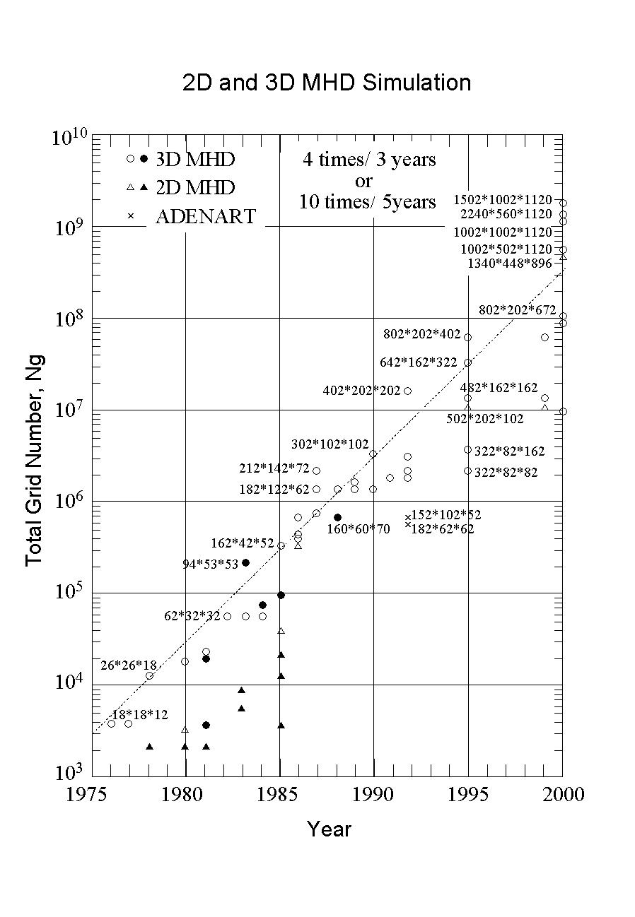
development and evaluate their future. Figure 3 shows a summary
plot of the 2 and 3-dimensional global MHD simulations indicating
how many grid points were used in each year. In this figure, the black
circles and triangles show the MHD simulations executed by other
groups, and the white ones and crosses show the MHD simulations
executed by our group. We began the 3-dimensional MHD simulations to
study MHD instabilities in toroidal plasmas using small number of grid
points given by 18*16*12 and 26*26*18 including the boundary in 1976.
However, the MHD simulations required about 50-200 hours of computing
time using a Fujitsu M-100 and M-200. The execution of such large scale
MHD simulations was practically limited by speed of the computers at that time.
We began a global MHD simulation of the earth's magnetosphere using a
larger number of grid points given by 62*32*32 and 50*50*26, including
the boundary using a CRAY-1 in 1982, when the memory of CRAY-1 of 1MW
limited the scale of the MHD simulation. At that time, we used to
consider how many interesting simulations could be executed if 100 cube
grid points could be used. The Japanese supercomputers subsequently
appeared, and we could execute the MHD simulations with 100 cube grid
points using Fujitsu VP-100, VP-200 and VP-2600. Later, we had a good
opportunity to use the Fujitsu VPP500 vector parallel machine in 1995
and began to use VPP5000 in 2000; this practically allowed us to
execute the MHD simulation with 1000 cube grid points. When we look
at the development of the MHD simulations from the point of view of the
number of grid points used in those 24 years, we can recognize the pattern
of a 4 fold increase every 3 years or a 10 fold increase every 5 years.
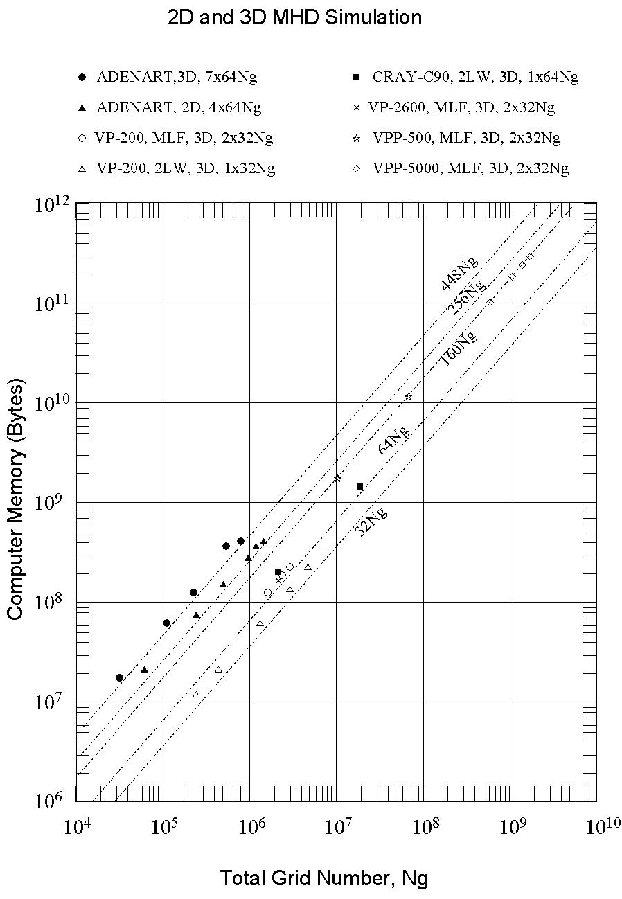
Figure 4 shows the computation time for an advance of one time step
which is needed to execute the MHD simulation, while Figure 5
shows the capacity of the computer memory which is needed to execute
the MHD simulation with the total grid points. The computation time
and capacity generally depend of the kind of computers and numerical
methods, and the computation time becomes longer and the necessary
computer memory increases in linear proportion to the number of total
grid points. Since the global MHD simulation of the earth's magnetosphere
requires repetitive calculations from several thousand to tens of thousands
times the one time step advance, it is necessary to make the computation time
of one time step advance less than 10 seconds in order to carry out practical
MHD simulations. Thus, the number of
usable grid points is automatically limited in MHD simulations by
the speed of the computers. At the same time the program size for MHD
simulations with the chosen grid points must be less than size of
the computer memory.
Since the time evolution of 8 physical components (i.e. the density,
3 components of velocity, plasma pressure and 3 components of magnetic
field) is calculated in the MHD code, the number of independent variables
is 8 Ng and the capacity is 32 Ng Bytes in single mode, where Ng is the
total grid number. Therefore, the key variables in the MHD code are 32 Ng
Bytes in the use of the 2 step Lax-Wendroff method (2LW)
and 64 Ng Bytes in the use of the modified Leap-Frog method (MLF)
because the MHD quantities must be stored at two time step intervals.
The 3-dimensional global MHD code which was originally developed for the
CRAY-1 and has been used by other vector machines requires only 1.3 times
the capacity to store the MHD key variables for a 1-dimensional array
in order to effectively decrease the work area. It becomes impossible
to effectively decrease the work area for parallel computers,
because the program size increases considerably in the parallel
machines such as ADENART, VPP500 and VPP5000. However the required
computer memory in VPP500 and VPP5000 is 2.5 times of capacity to
the key variables (160 Ng=2.5*64 Ng) in MLF. If the dependence on
required computer memory for the total grid number could be
concretely demonstrated, we could easily estimate how large an MHD
simulation could be executed to study specified subjects and could
establish more precisely the prospects for the future.
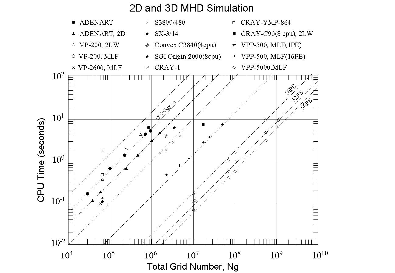
Figure 6 shows a comparison of the computer processing capability
with the total grid number in MHD simulations. Rapid progress has
been made in increasing performance by moving from a vector machine
to a vector parallel machine. Newer high performance workstations
and personal computers have the capability of older supercomputers
(speed of about 0.3 Gflops). However, the processing capability of
high end supercomputers keeps about a thousand times higher than that
of the other computers at all
times. Moreover, definitive differences between supercomputers and
other computers appear in the shortage of main memory and cache
required to carry out MHD simulations with a large number of grid
points. It is practically impossible to execute a 3-dimensional MHD
simulation code using workstations and personal computers when the
fully vectorized and fully parallelized MHD code would need cpu times
of 100 hours using a supercomputer such as VPP5000. It is now always
necessary to use a supercomputer with a maximum performance capability
in the study using 3-dimensional global MHD simulations of the
earth's magnetosphere.
5. Conclusions
We have executed a 3-dimensional global magnetohydrodynamic (MHD)
simulation of the interaction between the solar wind and the earth's
magnetosphere on a variety of computers using a fully vectorized MHD
code. However, simulation scientists have lost their common language
with appearance of vector parallel and massive parallel supercomputers.
We sincerely hope to see the development of a common language in the
supercomputer world. The candidates appear to be High Performance Fortran
(HPF) and Message Passing Interface (MPI). We look forward to the time when
we can use these compilers in supercomputers.
We have had the opportunity to use HPF/JA with a the Fujitsu VPP5000/56
supercomputer in the Computer Center of Nagoya University since last June.
We translated our 3-dimensional MHD simulation code for the Earth's
magnetosphere from VPP Fortran to HPF/JA and the code was fully vectorized
and fully parallelized in VPP Fortran. The performance of the HPF MHD code
was almost comparable to that of the VPP Fortran in a typical simulation using
a large number (56) of Processing Elements (PEs). Thus we have reached the
following conclusion: fluid and MHD codes that are fully vectorized and fully
parallelized in VPP Fortran can be relatively easily translated to HPF/JA,
and a code in HPF/JA can be expected to achieve comparable performance to one
written in VPP Fortran.
The 3-dimensional global MHD simulation code for the earth's magnetosphere
solves the MHD and Maxwell's equations in 3-dimensional Cartesian coordinates
(x, y, z) as an initial and boundary value problem using a modified leap-
frog method. The MHD quantities are distributed in the z direction. The
quantities in the neighboring grids can be calculated by the HPF/JA instruction
sentences "shadow" and "reflect" when they exist in another PE. Unnecessary
communication among PEs can be completely stopped by the instructions
"independent, new," and "on home, local." Moreover, the lump transmission of
data is used in the calculation of the boundary conditions by the instruction
"asynchronous." It was not necessary to change the fundamental structure of
the MHD code in the translation procedure. This was
a big advantage for translating the MHD code from VPP Fortran to HPF/JA.
Based on this experience, I anticipate that we will find little difficulty
in translating programs from VPP Fortran to HPF/JA, and we can expect an almost
comparable performance on the Fujitsu VPP5000. The maximum performance of
the 3-dimensional MHD code was over 230 Gflops for 32 PEs and over 400 Gflops
for 56 PEs. We hope that the MHD code rewritten in HPF/JA can be executed
on other supercomputers such as the Hitachi SR8000 and the NEC SX-5 in near
future and that HPF/JA becomes a real common language in the supercomputer world.
I believe that this is a necessary condition to restart a new and higher level
of collaborative research on 3-dimensional global MHD simulation of the
magnetosphere with other scientists around the world. I expect efforts by
simulation scientists as well as by the Japanese supercomputer companies to
reach this goal.
We have made available a part of the boundary condition in the HPF/JA MHD code
and a test program of the 3-dimensional wave equation at the following Web
address:
http://gedas.stelab.nagoya-u.ac.jp/simulation/hpfja/hpf01.html.
Acknowledgments. The work was supported by a grant in aid for science research
from the Ministry of Education, Science and Culture. Computing support was
provided by the Computer Center of Nagoya University.
References
Ogino, T., Magnetohydrodynamic simulation of interaction between the solar
wind and magnetosphere, J. Plasma and Fusion Research, (Review paper), Vol.75,
No.5, CD-ROM 20-30, 1999.
Ogino, T., Computer simulation of solar wind-magnetosphere interaction,
Center News, Computer Center of Nagoya University, Vol.28, No.4, 280-291, 1997.
Tsuda, T., On usage of supercomputer VPP5000/56,
Center News, Computer Center of Nagoya University, Vol.31, No.1, 18-33, 2000.
High Performance Fortran Forum, Official Manual of High Performance Fortran
2.0,
Springer, 1999.
Fujitsu Co., HPF programming -parallel programming (HPF version)-,
UXP/V Ver.1.0, June, 2000.
Fujitsu Co., VPP fortran programming, UXP/V, UXP/M Ver.1.2, April, 1997.
Table 1. Comparison of computer processing capability of VPP Fortran
and HPF/JA in a 3-dimensional global MHD code for the solar wind-magnetosphere
interaction using a Fujitsu VPP5000/56.
Figure Captions
Figure 1 Structure of 3-dimensional magnetic field lines for steady state
conditions in the earth's magnetosphere for an interplanetary magnetic field
which is northward and duskward. An asymmetry appears in the magnetosphere
due to the occurrence of magnetic reconnection on the dusk side in the northern
hemisphere and on the dawn side in the southern hemisphere near the
magnetopause. VRML1
Figure 2 An example of snapshots of the earth's magnetosphere obtained by
3-dimensional global MHD simulation, when the observational data of the solar
wind and interplanetary magnetic field obtained by the ACE satellite was used
as input for the simulation. VRML2
Figure 3 Development of 2 and 3-dimensional MHD simulations as quantified
by the total grid number used; the total grid number has increased 4 fold every
3 years or 10 fold every 5 years.
Figure 4 Comparison of computation times corresponding to an advance of one
time step versus total grid number in the MHD simulation codes.
Figure 5 Comparison of total capacity of the necessary computer memory versus
total grid number in the MHD simulation codes.
Figure 6 Comparison of the computer processing capability versus total grid
number in the MHD simulation codes.
Solar-Terrestrial Environment Laboratory, Nagoya University
(1) We can use the same domain division (z-direction in 3-dimension)
    as in VPP Fortran, and overlap data at the boundary of distributed
    data which was handled by "sleeve" in VPP Fortran can be replaced
    by "shadow" and "reflect" in HPF/JA.
(2) Parallelizing formalities for division are performed by
   "independent" sentence as is done in VPP Fortran.
(3) lump transmission of distributed data is done by "asynchronous"
    sentence.
(4) "asynchronous" sentence can be used for lump transmission between
    the distributed data with different divided directions.
(5) Unnecessary communication, which was problem in HPF, can be removed
    by instructions of "independent new(  )" and "on home local(  )".
(6) Maximum and minimum can be calculated in parallel by "reduction".
   Number of PEs:                               56 PE
   Theoretical maximum speed of PE:            9.6 Gflops
   Maximum memory capacity per PE for users:   7.5 GB
 Number    Number of     VPP Fortran               HPF/JA
 of PE     grids        cpu time  Gflops  Gf/PE   cpu time Gflops  Gf/PE

  1PE     200x100x478    119.607 (  0.17) 0.17 (scalar)
  1PE     200x100x478      2.967 (  6.88) 6.88       3.002 (  6.80) 6.80
  2PE     200x100x478      1.458 ( 14.01) 7.00       1.535 ( 13.30) 6.65
  4PE     200x100x478      0.721 ( 28.32) 7.08       0.761 ( 26.85) 6.71
  8PE     200x100x478      0.365 ( 55.89) 6.99       0.386 ( 52.92) 6.62
 16PE     200x100x478      0.205 ( 99.38) 6.21       0.219 ( 93.39) 5.84
 32PE     200x100x478      0.107 (191.23) 5.98       0.110 (186.13) 5.82
 48PE     200x100x478      0.069 (297.96) 6.21       0.074 (276.96) 5.77
 56PE     200x100x478      0.064 (319.53) 5.71       0.068 (299.27) 5.34

  1PE     500x100x200      2.691 (  7.94) 7.94       2.691 (  7.94) 7.94
  2PE     500x100x200      1.381 ( 15.47) 7.73       1.390 ( 15.37) 7.68
  4PE     500x100x200      0.715 ( 29.97) 7.47       0.712 ( 29.99) 7.50
  8PE     500x100x200      0.398 ( 53.65) 6.71       0.393 ( 54.38) 6.80
 16PE     500x100x200      0.210 (101.87) 6.37       0.202 (105.74) 6.61
 32PE     500x100x200      0.131 (163.55) 5.11       0.120 (175.50) 5.48
 48PE     500x100x200      0.100 (214.48) 4.46       0.091 (231.69) 4.82
 56PE     500x100x200      0.089 (239.48) 4.28       0.086 (244.85) 4.37

  4PE     800x200x670      7.618 ( 30.06) 7.52       8.001 ( 28.62) 7.16
  8PE     800x200x670      3.794 ( 60.36) 7.54       3.962 ( 57.81) 7.23
 12PE     800x200x670      2.806 ( 81.61) 6.80       3.005 ( 76.21) 6.35
 16PE     800x200x670      1.924 (119.00) 7.44       2.012 (113.85) 7.12
 24PE     800x200x670      1.308 (175.10) 7.30       1.360 (168.44) 7.02
 32PE     800x200x670      0.979 (233.85) 7.31       1.032 (221.88) 6.93
 48PE     800x200x670      0.682 (335.62) 6.99       0.721 (317.80) 6.62
 56PE     800x200x670      0.595 (384.61) 6.87       0.628 (364.87) 6.52

 16PE   1000x500x1118      9.668 (123.52) 7.72       9.619 (125.50) 7.84
 32PE   1000x500x1118      5.044 (236.73) 7.40       4.992 (241.83) 7.56
 48PE   1000x500x1118      3.550 (336.40) 7.01       3.479 (346.97) 7.23
 56PE   1000x500x1118      2.985 (400.04) 7.14       2.935 (411.36) 7.35
 32PE  1000x1000x1118      9.979 (239.33) 7.48       9.813 (243.37) 7.61
 48PE  1000x1000x1118      7.177 (332.79) 6.93       7.028 (339.85) 7.08
 56PE  1000x1000x1118      5.817 (410.55) 7.33       5.794 (412.23) 7.36
------------------------------------------------------------------------
 : Gflops is an estimated value for comparison with a computation by
   1 processor of a CRAY Y-MP C90
 STELab Home Page.